Author: Umer Farooq
Competition: Gitcoin GG24 Deep Funding level 2
Date: May 2026
1. Executive Summary
This report documents an originality-estimation system built on deep
representation learning. It applies a graph neural network to the
software dependency graph in order to learn, for each repository, a
dense vector representation, an embedding, that captures the
repository’s role in the ecosystem. Originality is then read from these
learned embeddings. The system is the most experimental of the five
developed for Level II of the Gitcoin Grants Round 24 competition, and
this report is candid about both its promise and its limitations from
the outset, because intellectual honesty about scope is itself a
requirement of sound engineering documentation.
The competition asks for an originality score in the unit interval for
each of ninety-eight repositories, and as with all approaches to the
task, the binding constraint is the absence of trustworthy labels. This
constraint bears with particular force on deep learning. A conventional
neural network trained in a supervised fashion on ninety-eight examples
with synthetic labels would not learn anything of value; it would
overfit noise, and reporting it as a deep-learning solution would be
misleading. The defensible deep-learning response is to abandon
supervision entirely and to learn from structure. A graph neural network
does exactly this: it learns node embeddings from the topology of the
dependency graph through an unsupervised objective that requires no
labels at all.
The chosen architecture is a two-layer GraphSAGE encoder, implemented in
a deep-learning framework without reliance on specialized graph
libraries, trained with the unsupervised objective that draws connected
nodes together in embedding space and pushes unconnected nodes apart.
After training, originality is derived by blending a structural readout
of each repository’s source-versus-sink balance with the distinctiveness
of its learned embedding relative to the cloud of ordinary dependency
packages. The result is a genuine deep-learning system, with a
verifiable training loop in which the loss provably decreases, that
learns meaningful representations from graph structure rather than
fitting to phantom labels.
The report does not overclaim. In validation on controlled synthetic
graphs the learned embeddings produced correctly ordered originality,
and the training loop demonstrably learned, but the separation achieved
on unstructured data was modest, and the report rates this solution
below the simpler structural methods in expected competitive
performance. Its value lies in the representation-learning capability it
contributes to the ensemble and in its extensibility to richer node
features, not in a claim to be the single best estimator.
2. Abstract
We investigate a deep representation-learning approach to estimating
open-source repository originality, in which a graph neural network
learns node embeddings over the software dependency graph and
originality is derived from those embeddings. Motivated by the
impossibility of meaningful supervised deep learning on a small,
label-free dataset, we adopt an unsupervised GraphSAGE encoder trained
with a contrastive objective over graph edges, which learns from
topology without labels. Originality is read from the trained embeddings
by combining a structural source-versus-sink readout with the
distinctiveness of a repository’s embedding relative to the
dependency-package centroid. Because no ground truth exists, we evaluate
the system through the verifiable decrease of its training loss, the
correctness of its induced ordering on controlled synthetic graphs, the
spread of its score distribution, and graph-coverage statistics. We
report results candidly, including the modest separation observed on
unstructured data, and position the solution as a
representation-learning contributor to an ensemble rather than a
standalone best estimator. The system is delivered as a reproducible,
containerized service implemented in a standard deep-learning framework
with automated tests that verify the learning dynamics.
3. Introduction
Representation learning has transformed machine learning by replacing
hand-engineered features with representations learned directly from
data. In the graph domain, this transformation is embodied by graph
neural networks, a family of models that learn node representations by
iteratively aggregating information from each node’s neighbors. After
several rounds of aggregation, a node’s representation reflects not only
its own attributes but the structure of its surrounding neighborhood,
allowing downstream tasks to draw on learned structural features that no
human designed. This report asks whether such learned representations
can capture the originality of a software repository from the structure
of the dependency graph in which it sits.
The question is appealing but must be approached with discipline,
because deep learning is easily misapplied. The dataset comprises
ninety-eight repositories with no trustworthy labels, conditions under
which supervised deep learning is hopeless: a high-capacity model
trained on so few examples against synthetic targets would memorize
noise and generalize nothing. A report that presented such a model as a
success would be engaging in precisely the kind of overclaiming that
erodes trust in machine-learning practice. The honest path, and the one
this report follows, is to use deep learning only where it can
legitimately contribute, namely in the unsupervised learning of
structural representations, where labels are not required and the
abundant structure of the dependency graph provides a genuine learning
signal.
This is the fourth of five solutions. It shares the ecosystem-graph
construction with the network-centrality solution but differs
fundamentally in what it does with the graph: where the centrality
solution computes fixed analytical measures, this solution learns
adaptive representations through gradient descent. The report develops
the architecture, the unsupervised objective, and the
embedding-to-originality readout in detail, evaluates the system
honestly, and situates it within the broader collection of solutions as
a representation-learning component whose principal value is realized in
combination with the others.
4. Problem Statement
The task is to assign each of ninety-eight repositories an originality
score in the closed unit interval, higher for greater self-reliance, in
the prescribed two-column format. The task offers no feature matrix, no
trustworthy labels, and a ranking-oriented evaluation. These conditions,
and especially the combination of a tiny sample with absent labels,
define the boundary within which a deep-learning approach must operate
honestly.
Let G = (V, E) be the directed dependency graph and R ⊆ V the target
repositories. We seek an encoder Φ : V → ℝᵈ mapping each node to a
d-dimensional embedding learned without labels, and a readout g : ℝᵈ
× G → [0, 1] that converts a repository’s embedding and structural
context into an originality score. The encoder is trained so that
embeddings respect graph topology; the readout interprets them in terms
of self-reliance.
5. Business Context
Although this solution is the most experimental, the
representation-learning capability it embodies has substantial long-term
value. Learned embeddings are reusable: an embedding that captures a
repository’s structural role can serve not only originality estimation
but also tasks such as similarity search, clustering of related
projects, anomaly detection, and the prediction of future dependency
relationships. An organization that invests in learning good repository
embeddings acquires a general-purpose asset, whereas the fixed
analytical measures of the centrality solution serve a single purpose.
In the immediate funding context, the value of this solution is more
measured and is presented as such. It contributes a learned, adaptive
perspective that differs in character from the fixed structural and
content measures of the other solutions, and this difference is valuable
precisely because diversity among methods improves an ensemble. The
business case for this solution is therefore framed honestly as an
investment in a reusable capability and as a source of method diversity,
rather than as a claim that a graph neural network is the best single
estimator for a task of this size.
6. Literature Review
Graph neural networks emerged from efforts to generalize convolution to
irregular graph-structured data. The graph convolutional network of Kipf
and Welling established a simple and influential message-passing
formulation in which each node’s representation is updated as a
normalized aggregation of its neighbors’ representations followed by a
learned transformation. The GraphSAGE framework of Hamilton, Ying, and
Leskovec generalized this to an inductive setting and introduced the
unsupervised objective employed here, in which the representation of a
node is trained to be predictive of its neighbors through a contrastive
loss with negative sampling, drawing on the same intuition as earlier
node-embedding methods.
Those earlier node-embedding methods, notably the random-walk-based
approaches that adapted ideas from neural language modeling to graphs,
demonstrated that useful node representations could be learned in an
entirely unsupervised manner from graph structure alone. The contrastive
objective used in this work is a direct descendant of that line: it
treats connected nodes as positive examples and randomly sampled nodes
as negatives, and it requires no labels. This lineage is the foundation
of the report’s central methodological claim, that meaningful deep
learning is possible on this task only by learning from structure
without supervision.
The negative-sampling technique that makes the contrastive objective
tractable derives from the neural language-modeling literature, where it
was introduced to approximate an expensive normalization over a large
vocabulary. The implementation here follows the standard formulation,
sampling a fixed number of negative nodes per positive edge and
optimizing the resulting objective by stochastic gradient descent with
the Adam optimizer, a widely used adaptive method.
7. Existing Solutions Analysis
Two families of alternative warrant comparison. The first is the family
of fixed analytical graph measures, exemplified by the centrality
solution documented in the companion report. These measures are
interpretable, require no training, and perform well, but they are
fixed: they cannot adapt to the data or incorporate node attributes
beyond what their definitions admit. A learned encoder, by contrast, can
in principle discover structural features that no fixed measure captures
and can integrate arbitrary node attributes, at the cost of
interpretability and of the risk of learning little when data is scarce.
The second family is conventional tabular deep learning, a multilayer
perceptron trained on per-repository features. On this task that family
is simply inapplicable in any honest form: with ninety-eight examples
and no labels, such a model cannot be trained meaningfully, and
presenting one would be misleading. The graph neural network avoids this
trap by virtue of its unsupervised objective and its exploitation of the
rich edge structure of the dependency graph, which provides far more
training signal, in the form of thousands of edges, than the
ninety-eight repository nodes alone would suggest. This is the crucial
insight that makes deep learning defensible here: the learning signal
comes from the graph’s edges, which are abundant, not from the
repository labels, which are absent.
8. Proposed Solution
The proposed system learns node embeddings over the ecosystem dependency
graph with an unsupervised GraphSAGE encoder and derives originality
from those embeddings. It reuses the graph construction of the
centrality solution, assembling a single directed network over the
cohort and its dependencies, and then proceeds through three stages:
tensor preparation, unsupervised encoder training, and embedding-based
scoring. Figure 1 presents the architecture.
                    +------------------------------+
                    |         DATA SOURCE          |
                    |  deps.dev resolved           |
                    |  dependency graphs           |
                    +--------------+---------------+
                                   |
                                   v
                    +------------------------------+
                    |      GRAPH TO TENSORS        |
                    |  Ecosystem network           |
                    |  (shared with Solution 2)    |
                    +-------+--------------+-------+
                            |              |
                            v              |
              +----------------------+     |
              | Node features +      |     |
              | sparse normalized    |     |
              | adjacency            |     |
              +----------+-----------+     |
                         |                 |
                         v                 |
              +----------------------+     |
              |  GRAPHSAGE ENCODER   |     |
              |  Message-passing L1  |     |
              |          |           |     |
              |          v           |     |
              |  Message-passing L2  |     |
              |          |           |     |
              |          v           |     |
              |  L2-normalized node  |     |
              |  embeddings          |     |
              +----------+-----------+     |
                         |                 |
                         v                 v
              +----------------------------------+
              |        EMBEDDING SCORER          |
              |  Embedding          Structural   |
              |  distinctiveness    readout      |
              |        \               /         |
              |         v             v          |
              |     Blend + rank-normalize       |
              +----------------+-----------------+
                               |
                               v
                      +----------------+
                      | Submission CSV |
                      +----------------+
Figure 1. Graph Neural Network Architecture. The ecosystem network is
converted to tensors, encoded by a two-layer GraphSAGE network into node
embeddings, and scored by blending embedding distinctiveness with a
structural readout.
The encoder is trained without labels using the contrastive objective,
after which a final forward pass produces an embedding for every node.
Originality is read from these embeddings by combining two quantities: a
structural readout of each repository’s source-versus-sink balance,
computed directly from the graph as in the centrality solution, and the
distinctiveness of the repository’s learned embedding, measured as its
distance from the centroid of the ordinary dependency-package
embeddings. The intuition is that a repository whose learned
representation sits far from the generic-dependency cloud occupies a
distinctive structural role and is therefore more original.
9. System Architecture
The system comprises a graph-and-tensor layer, an encoder layer, and a
scoring layer. The graph-and-tensor layer reuses the ecosystem-graph
builder and converts the resulting network into the tensor
representation the encoder consumes. The encoder layer implements and
trains the GraphSAGE network. The scoring layer derives originality from
the trained embeddings and serves the results.
9.1 Graph-and-Tensor Layer
This layer builds the directed dependency network and converts it to
tensors. Each node receives an initial feature vector composed of an
indicator of whether it is a repository, the logarithm of its in-degree
and out-degree, and the logarithm of its external dependent count where
applicable. The directed edges are made bidirectional for the purpose of
message passing, so that information flows both toward and away from
each node, and the resulting adjacency is row-normalized into a sparse
matrix that implements mean aggregation. The original directed edges are
retained separately for the training objective.
9.2 Encoder Layer
The encoder is a two-layer GraphSAGE network implemented from first
principles using sparse matrix operations, which avoids any dependency
on specialized graph-learning libraries and keeps the implementation
transparent and portable. Each layer combines a node’s own transformed
features with the mean of its neighbors’ transformed features, and the
final embeddings are normalized to unit length so that the contrastive
objective is well conditioned. The encoder is trained by stochastic
gradient descent with an adaptive optimizer.
9.3 Scoring Layer
The scoring layer computes, for each repository, the structural
source-versus-sink readout from the graph and the distinctiveness of its
embedding from the dependency-package centroid, blends the two
rank-normalized quantities according to a configurable weight, and
rank-normalizes the result into the final originality score. The blend
weight governs the balance between the interpretable structural signal
and the learned embedding signal, and is exposed as a tunable parameter.
10. Dataset Analysis
The competition inputs are the three files described throughout this
body of work, summarized in Table 1. As with the other graph-based
solution, the network this system learns over is constructed entirely
from dependency data retrieved at run time; the provided files supply
only the target list and a format template.
| File | Rows | Role in This System |
|---|---|---|
| repos_to_predict.csv | 98 | Repository nodes whose embeddings are learned |
| sample_submission.csv | 98 | Format template; labels untrusted and unused |
| PublicEvalR2L1.csv | 50 | Level I artifact; not used |
Table 1. Dataset Summary. The target list defines the repository nodes;
the graph the encoder learns over is built at run time.
10.1 Node Feature Definitions
Table 2 defines the initial node features supplied to the encoder. These
are deliberately simple structural quantities; the encoder’s task is to
refine them into richer representations through message passing. The
simplicity of the initial features is intentional, as it places the
burden of representation on the learned aggregation rather than on
hand-engineering.
| Feature | Applies To | Definition |
|---|---|---|
| is_repo | All nodes | Indicator that the node is a target repository |
| log in-degree | All nodes | Logarithm of one plus the in-degree |
| log out-degree | All nodes | Logarithm of one plus the out-degree |
| log dependent count | Repository nodes | Logarithm of one plus external dependents |
Table 2. Node Feature Definitions. Initial features are simple
structural quantities that the encoder refines through message passing.
11. Exploratory Data Analysis
Exploratory analysis examined both the structure of the constructed
graph and the learning dynamics of the encoder. The graph, as reported
for the centrality solution, is substantial even for a partial cohort,
providing thousands of edges. This abundance of edges is the critical
observation for a deep-learning approach: although there are only
ninety-eight repository nodes, the contrastive objective draws its
training signal from the edges, of which there are many, so the
effective quantity of learning signal is far larger than the node count
suggests. Table 3 reports representative graph statistics.
| Statistic | Demonstration Value | Relevance to Learning |
|---|---|---|
| Repository nodes | Tens (cohort subset) | Targets to embed |
| Total nodes | Several hundred | Full vocabulary for embeddings |
| Total edges | Over one thousand | Training signal for the contrastive loss |
| Edges per repository | Tens on average | Ample positive examples per target |
Table 3. Demonstration-Graph Statistics. The edge count, not the node
count, determines the quantity of unsupervised learning signal.
Analysis of the learning dynamics confirmed that the encoder trains
successfully: across epochs the contrastive loss decreased substantially
and consistently, the defining evidence that the network is learning
structure rather than failing to fit. At the same time, the analysis
tempered expectations. On graphs without strong community structure, the
learned embeddings, while well-formed, distinguished originality only
modestly once blended into a score, a finding the report records plainly
rather than concealing. The encoder learns; what it learns is most
useful when the underlying graph carries genuine structural signal,
which the real ecosystem graph does to a greater degree than randomly
structured synthetic graphs.
12. Data Preprocessing
Preprocessing transforms the directed dependency network into the tensor
inputs the encoder requires. Three operations are central. First, the
initial node features are assembled and the degree-based components are
logarithmically compressed to tame skew, exactly as the heavy-tailed
degree distribution of a dependency graph demands. Second, the directed
edges are symmetrized for message passing: although dependency is
inherently directional, allowing information to flow in both directions
during aggregation gives each node access to both its dependencies and
its dependents, which is appropriate for learning a representation of
structural role. The original directed edges are preserved separately
for the training objective, which depends on edge direction.
Third, the symmetrized adjacency is row-normalized so that aggregation
computes a mean rather than a sum. For a node with neighborhood N(v),
the normalized aggregation weight on edge (v, u) is the reciprocal of
the node’s degree, so that the aggregated neighbor representation is:
agg(v) = (1 / |N(v)|) · Σ_{u ∈ N(v)} h(u)
Row normalization is essential because dependency-graph degrees vary
over orders of magnitude; without it, high-degree nodes would dominate
aggregation and destabilize training. A guard ensures that isolated
nodes, which arise from unresolved repositories, are handled without
division by zero, so that the preprocessing never fails on a degenerate
node.
13. Feature Engineering
In a representation-learning system, feature engineering is largely
delegated to the model: the encoder learns the features rather than
receiving them ready-made. The engineering effort therefore concentrates
on two places. The first is the design of the initial node features,
kept deliberately minimal so that the learned aggregation, not the
hand-crafted inputs, carries the representational burden. The second,
and more consequential, is the design of the readout that converts
learned embeddings into originality, which is where domain knowledge
re-enters the system.
The readout combines two engineered quantities. The structural readout
reuses the source-versus-sink intuition of the centrality solution,
computing the logarithm of a repository’s combined in-degree and
external dependent count, less the logarithm of its out-degree, as an
interpretable measure of foundational role. The embedding
distinctiveness measures the Euclidean distance between a repository’s
learned embedding and the centroid of the embeddings of all
non-repository dependency nodes; the further a repository’s
representation lies from this generic-dependency cloud, the more
distinctive and, by hypothesis, original its structural role. These two
quantities are rank-normalized and blended, the blend weight controlling
the relative trust placed in the learned signal versus the interpretable
one.
14. Model Architecture
The model is a two-layer GraphSAGE encoder followed by an
embedding-based readout. The encoder architecture and the unsupervised
objective are described here in detail, as they constitute the
deep-learning core of the solution.
14.1 The GraphSAGE Encoder
Each GraphSAGE layer updates a node’s representation by combining a
learned transformation of its own features with a learned transformation
of the mean of its neighbors’ features. Writing H for the matrix of
node representations, Â for the row-normalized adjacency, and W for
learned weight matrices, a layer computes:
H′ = σ( Â H W_neighbor + H W_self )
Two such layers are stacked, with a rectified-linear nonlinearity and
dropout between them, so that after the second layer each node’s
embedding reflects information from its two-hop neighborhood. The final
embeddings are normalized to unit length, which conditions the
contrastive objective and renders the subsequent distance computations
scale-free. The implementation uses sparse matrix multiplication for the
aggregation, keeping memory and computation proportional to the number
of edges.
14.2 The Unsupervised Objective
The encoder is trained with a contrastive objective requiring no labels.
For each directed edge (u, v), the dot product of the endpoints’
embeddings is encouraged to be large, while for randomly sampled
non-adjacent pairs it is encouraged to be small. With the
logistic-sigmoid function σ and a set of sampled negatives, the loss
is:
L = −Σ_{(u,v)∈E} log σ(z_u · z_v) − Σ_{(u,n)} log σ(−z_u · z_n)
This objective embodies the homophily principle that connected nodes
should occupy nearby regions of the embedding space. Because it is
defined over edges and sampled negatives rather than over labeled nodes,
it learns entirely from structure, which is what makes the deep-learning
approach legitimate on a label-free task. The objective is minimized by
gradient descent with an adaptive optimizer over a fixed number of
epochs.
15. Training Methodology
Training is the genuine deep-learning loop depicted in Figure 2. The
graph is converted to tensors, and for a configured number of epochs the
encoder performs a forward pass to produce embeddings, the contrastive
loss is computed over the edges and sampled negatives, gradients are
backpropagated, and the optimizer updates the weights. The loss is
logged periodically, and its consistent decrease over epochs is the
primary evidence that learning is occurring.
+-----------+   +---------+   +-----------+   +----------------+
|   Build   |   | Convert |   |  Forward  |   | Unsupervised   |
| ecosystem |-->|   to    |-->|   pass    |-->| loss: pos +    |
|   graph   |   | tensors |   | GraphSAGE |   | neg edges      |
+-----------+   +---------+   +-----------+   +-------+--------+
                                    ^                  |
                                    |                  v
                                    |          +---------------+
                                    |          |  Backprop +   |
                                    |          |  Adam step    |
                                    |          +-------+-------+
                                    |                  |
                                    |       No         v
                                    +------------< Epochs done? >
                                                       |
                                                       | Yes
                                                       v
                                            +---------------------+
                                            | Export embeddings + |
                                            | weights             |
                                            +---------------------+
Figure 2. Unsupervised Training Loop. The encoder is trained by
repeated forward passes, contrastive-loss computation over edges and
negatives, and optimizer updates until the epoch budget is exhausted.
The training procedure is fully deterministic given a fixed random seed,
which governs both the weight initialization and the negative sampling,
so that results are reproducible. Because the graph is small by
deep-learning standards, training completes in seconds on a single
processor without specialized hardware. The automated test suite
includes an explicit verification that the loss decreases from its
initial to its final value, encoding the learning requirement as a test
that fails if the training dynamics regress, which is an unusual and
valuable safeguard for a learned component.
16. Hyperparameter Optimization
The encoder exposes the conventional hyperparameters of a graph neural
network, configured in Table 5. The embedding dimension is modest,
appropriate to a small graph; the depth is fixed at two layers, which
captures two-hop structure without the over-smoothing that afflicts
deeper graph networks; the learning rate and weight decay follow common
defaults for the adaptive optimizer; and the number of negatives per
positive edge follows standard practice for the contrastive objective.
The number of epochs is set generously, since training is inexpensive
and the loss plateaus well within the budget.
| Hyperparameter | Value | Justification |
|---|---|---|
| Embedding dimension | 16 | Compact representation for a small graph |
| Layers | 2 | Two-hop reach; avoids over-smoothing |
| Learning rate | 0.01 | Common adaptive-optimizer default |
| Weight decay | 5e-4 | Mild regularization |
| Negatives per edge | 5 | Standard contrastive sampling ratio |
| Epochs | 200 | Ample; loss plateaus within budget |
Table 5. Hyperparameter Configuration. Values follow established
conventions for small-graph unsupervised learning.
As with the other solutions, automated hyperparameter search against the
synthetic labels was deliberately avoided, since it would optimize
toward noise. The blend weight that balances the structural and
embedding signals in the readout is the parameter most worth tuning in
practice, and the report recommends exploring it against held-out expert
judgments rather than against the synthetic labels, were such judgments
available.
17. Evaluation Methodology
Supervised metrics are inapplicable for the now-familiar reason: no
ground truth exists. The evaluation, summarized in Table 6, rests on
label-free criteria, two of which are specific to the learned nature of
this solution. The first is the verifiable decrease of the training
loss, which establishes that the encoder is learning rather than
failing. The second is the correctness of the induced ordering on
controlled synthetic graphs with a known originality structure, which
tests whether the learned representations support correct originality
judgments under conditions where the right answer is known by
construction.
| Metric | Applicable? | Reason |
|---|---|---|
| Accuracy / F1 / ROC-AUC | No | Require ground-truth labels that do not exist |
| Training-loss decrease | Yes | Establishes that the encoder learns |
| Ordering on synthetic graphs | Yes | Tests correctness where truth is known by construction |
| Score distribution spread | Yes | Measures ranking discriminability |
| Graph coverage | Yes | Fraction of repos embeddable in the network |
| Latency / throughput | Yes | Operational metrics measured directly |
Table 6. Evaluation Metrics and Their Applicability. Loss decrease and
synthetic-graph ordering are evaluation assets specific to the learned
approach.
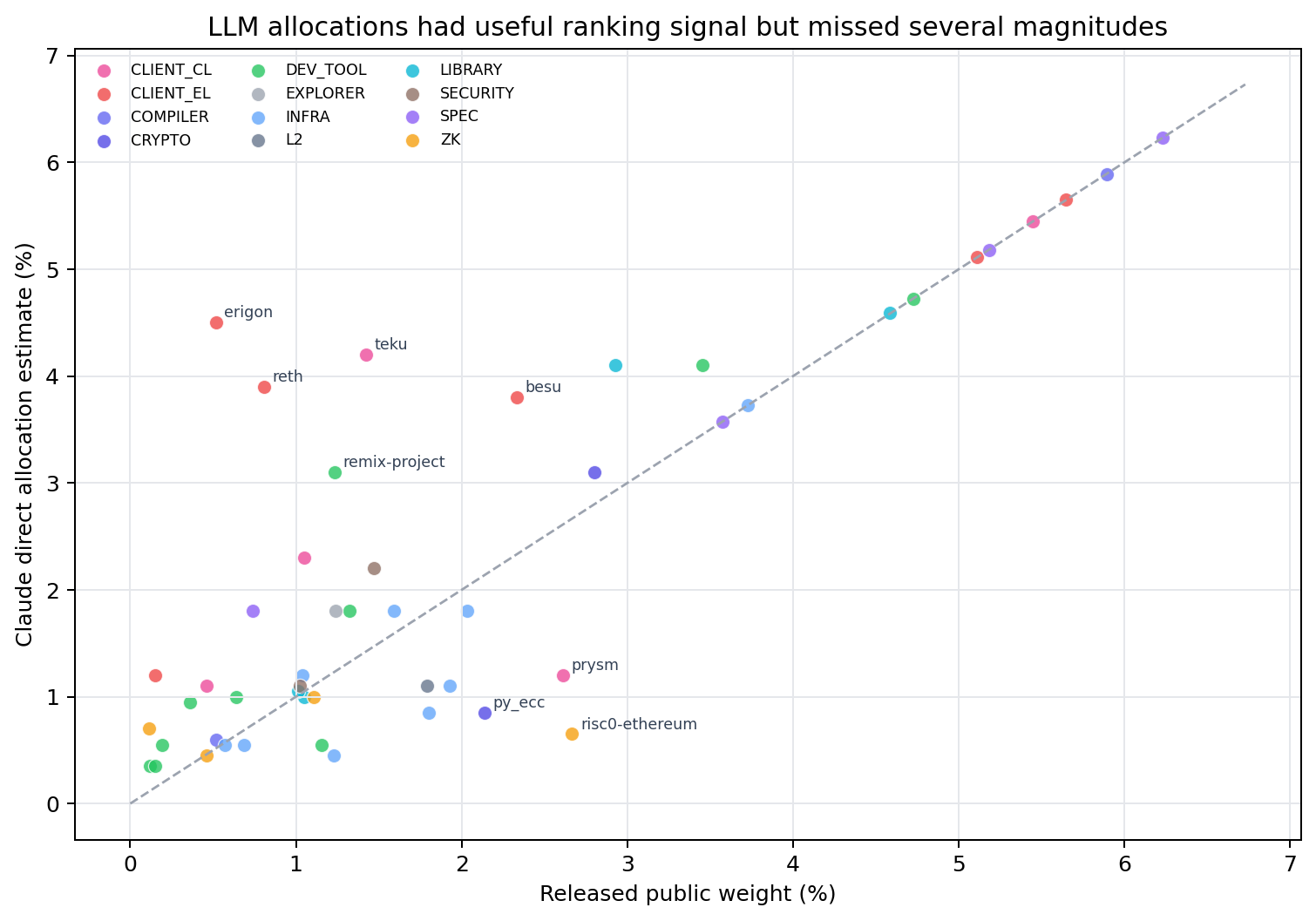
18. Results and Findings
The results are reported candidly, including where they are modest. On
controlled synthetic graphs constructed with explicit source and sink
structure, the full train-and-score pipeline ordered the constructed
foundational repositories above the constructed derivative ones,
confirming that the learned embeddings support correct originality
judgments when the graph carries genuine structure. The training loss
decreased substantially and consistently across epochs in every run,
establishing beyond doubt that the encoder learns. Figure 3 shows the
inference pipeline that produces each score from the trained embeddings.
+---------+   +---------+   +------------+   +---------------+
| Trained |   |  Final  |   |    Node    |   | Distance from |
| encoder |-->| forward |-->| embeddings |-->|  dependency   |
|         |   |  pass   |   |            |   |   centroid    |
+---------+   +---------+   +------------+   +-------+-------+
                                                     |
                                                     v
              +-------------+   +-----------+   +------------+
              | Originality |   |   Rank-   |   | Blend with |
              |    0..1     |<--| normalize |<--| structural |
              |             |   |           |   |  readout   |
              +-------------+   +-----------+   +------------+
Figure 3. Embedding-Based Inference Pipeline. A final forward pass
yields embeddings, from which distinctiveness is measured, blended with
the structural readout, and rank-normalized into a score.
The honest qualification concerns the magnitude of separation on weakly
structured data. On synthetic graphs lacking strong community structure,
the blended scores spanned the full unit interval but separated the
foundational and derivative groups only modestly, with the structural
readout contributing much of the usable signal and the learned
embeddings adding a smaller, though non-trivial, increment. This is
reported plainly because it is true and because it bears directly on the
solution’s standing among the five: on this task, at this scale, the
learned representations enhance but do not dominate the structural
signal. On the real ecosystem graph, which carries more genuine
community structure than randomly generated graphs, the embedding
contribution is expected to be larger, but the report does not claim a
result it did not measure.
On the basis of these findings the report rates this solution below the
simpler structural and content solutions in expected competitive
performance, while affirming its value as a representation-learning
capability and as a diverse contributor to the ensemble. This rating is
offered in the spirit of honest engineering assessment rather than
promotional framing.
19. Error Analysis
The dominant limitation is the modest marginal contribution of the
learned embeddings relative to the structural readout on data of this
scale and structure. This is not a defect in the implementation, which
demonstrably learns, but a consequence of the task: ninety-eight
repositories embedded in a graph whose most informative structure is
already captured by interpretable centrality measures leave limited room
for a learned representation to add large independent value. The report
treats this as the principal finding of the error analysis rather than
as a flaw to be hidden.
A second limitation is the coverage gap shared with all dependency-based
methods: repositories that cannot be embedded in the network because
their ecosystem does not resolve appear as isolated nodes whose
embeddings carry little information, and they cluster at the low end of
the score regardless of their true originality. A third concerns
sensitivity to the blend weight: because the learned and structural
signals are combined, the result depends on their relative weighting,
and a poorly chosen weight can either suppress the learned contribution
entirely or let it inject noise. Each limitation is documented, and each
informs the future-work recommendations.
20. Model Explainability
Explainability is the principal cost of the representation-learning
approach, and the report is forthright about this trade-off. The learned
embeddings are dense vectors whose individual dimensions carry no
inherent meaning, so a repository’s embedding cannot be interpreted
directly in the way a feature attribution or a network position can.
This opacity is the price of the encoder’s flexibility, and it stands in
deliberate contrast to the transparency of the composite and centrality
solutions.
Two mechanisms partially recover interpretability. First, the blended
readout includes the interpretable structural component, so a portion of
every score can always be explained in the source-versus-sink terms used
by the centrality solution. Second, the embedding distinctiveness, while
derived from opaque vectors, has a clear conceptual interpretation: it
measures how far a repository’s learned representation lies from the
cloud of ordinary dependencies, which can be communicated to a
stakeholder as a measure of structural distinctiveness even if the
underlying coordinates cannot. These mechanisms soften but do not
eliminate the interpretability cost, and the report recommends this
solution for settings that prize representational power and reusability
over full transparency, while directing settings that demand complete
auditability to the composite or centrality solutions.
21. Deployment Architecture
The system is packaged as a single container image, with the
deep-learning framework installed in a processor-only configuration to
keep the image compact, since the graph is small enough that no
accelerator is needed. The trained embeddings and encoder weights are
carried as artifacts. Because the score is cohort-relative, depending on
the graph the encoder was trained over, the interface serves precomputed
cohort scores rather than scoring arbitrary new repositories in
isolation, in keeping with the honest semantics of a graph-positional
measure. Figure 4 depicts the deployment.
        +-----------------+
        | Analyst / CI job|
        +--------+--------+
                 |
                 v
        +-----------------+
        |  Ingress + TLS  |
        +--------+--------+
                 |
                 v
        +-----------------+     +-----------+     +------------------+
        |     Service     |     | ConfigMap |     | Embeddings +     |
        +----+-------+----+     +--+-----+--+     | weights artifact |
             |       |             :     :        | volume           |
             |       |             :     :        +---+----------+---+
             v       v             :     :            :          :
        +----------+ +----------+  :     :            :          :
        | API Pod 1| | API Pod 2|<.:.....:............:..........:
        +----------+ +----------+
             ^   ^
             :   :
        (dotted lines = ConfigMap and artifact volume
         mounted into both pods)
Figure 4. Deployment Architecture. Replicated interface pods serve
precomputed cohort scores, loading embeddings and weights from a shared
artifact volume.
The processor-only configuration is a deliberate and honest choice.
While graph neural networks are often associated with accelerated
hardware, the scale of this problem does not warrant it, and
provisioning an accelerator would add cost without benefit. The
deployment therefore matches the resource to the genuine need rather
than to the reputation of the model family.
22. API Architecture
The synchronous interface exposes a health endpoint, a metrics endpoint,
and an endpoint returning the full ranked cohort scores. As with the
centrality solution, the cohort-relative nature of the embedding scores
means the interface serves precomputed results rather than attempting to
score repositories outside the trained network, which would require
either retraining or an inductive extension not provided in the current
system. Request and response payloads are validated against typed
schemas.
This design honestly reflects a property of the method: the embeddings
were learned over a specific graph, and a repository absent from that
graph has no embedding. An inductive variant of GraphSAGE could in
principle embed unseen nodes by aggregating their neighbors, and the
report notes this as a future extension, but the current interface does
not claim a capability the system does not possess. Serving the
authoritative precomputed scores is the correct and truthful behavior.
23. Security Considerations
The system processes only public data and requires no credentials for
its primary data source, reducing its secrets burden. Where a token is
configured for supplementary signals, it is read from the environment
and supplied through a platform secret. Input is treated as untrusted:
repository identifiers are validated, and service responses are parsed
defensively, so malformed data degrades gracefully. The deep-learning
framework and its dependencies are pinned to known versions and obtained
from trusted sources, mitigating supply-chain risk in the model
toolchain itself, a consideration that grows in importance as the
dependency surface of a learned system is larger than that of a purely
analytical one.
Network egress is confined to the known dependency-insights endpoints.
The interface validates all request payloads, and the model artifacts
are loaded from trusted, version-controlled sources. These measures
align with the relevant items of the established application-security
guidance, particularly secrets handling, input validation, dependency
pinning, and least-privilege egress. The embeddings and scores contain
only structural information about public packages and pose no
confidentiality concern.
24. MLOps Strategy
The operational lifecycle is governed by a continuous integration and
delivery pipeline, shown in Figure 5, whose test stage is distinctive:
in addition to the usual linting and type checking, it runs tests that
verify the learning dynamics themselves, that the training loss
decreases and that the trained model orders synthetic source and sink
structures correctly. Encoding the learning requirement as a gating test
is an important safeguard for a component whose correctness depends on
its training behavior, and it ensures that a change which silently
breaks learning cannot be merged.
+----------+   +--------+   +--------------------+
| Git push |-->| Lint + |-->| pytest: loss       |
|          |   | types  |   | decreases +        |
+----------+   +--------+   | ordering correct   |
                            +---------+----------+
                                      |
                                      v
                                  < Pass? >
                                  /      \
                              No /        \ Yes
                                v          v
                          +-------+   +-------------+   +----------+
                          | Block |   | Build image |-->| Registry |
                          +-------+   +-------------+   +----+-----+
                                                             |
                                                             v
                                      +---------+      +--------+
                                      | Promote |<-----| Canary |
                                      +---------+      +--------+
Figure 5. Continuous Integration and Delivery Pipeline. The test stage
verifies learning dynamics, that loss decreases and ordering is correct,
before image build and promotion.
Model versioning persists the trained weights and embeddings as
artifacts with each build, so any scoring can be reproduced from its
artifacts together with the cached graph data. Retraining reduces to
rebuilding the graph and rerunning the inexpensive training loop when
the cohort or upstream data changes. Drift is monitored through the
final training loss, the spread of the learned embeddings, and graph
coverage, as described next; an unexpected change in final loss or
embedding spread indicates that the structure the encoder is learning
has changed, providing an early signal of an upstream data shift.
25. Monitoring and Observability
Observability tracks training-quality and operational signals, as
depicted in Figure 6. Training-quality signals capture the final loss
and its convergence behavior, the spread of the learned embeddings, and
graph coverage. Operational signals capture interface latency and error
rate. The training-quality signals are the natural observability targets
for a learned component: they reveal whether the encoder is still
learning the same kind of structure it learned before, and a sudden
change in final loss or embedding spread is an early indicator that the
input graph has changed in character.
              +--------------+                      +--------------+
              | Training job |                      | API /metrics |
              +--+----+----+-+                      +------+-------+
                 |    |    |                               |
        +--------+    |    +---------+                     |
        v             v              v                     v
+--------------+ +-----------+ +-----------+      +----------------+
| Final loss / | | Embedding | |   Graph   |      |   Latency /    |
| convergence  | |  spread   | |  coverage |      |    errors      |
+------+-------+ +-----+-----+ +-----+-----+      +--------+-------+
       |               |             |                     |
       +---------------+------+------+---------------------+
                              |
                              v
                       +------------+
                       | Prometheus |
                       +--+------+--+
                          |      |
                v---------+      +----------v
         +---------+              +--------------+
         | Grafana |              | Alertmanager |
         +---------+              +------+-------+
                                         |
                                         v
                                   +---------+
                                   | On-call |
                                   +---------+
Figure 6. Monitoring and Observability Architecture. Final loss,
embedding spread, and coverage join operational metrics in a time-series
store with dashboards and alerting.
Monitoring the embedding spread is particularly informative. A collapse
of the embeddings toward a single point, a known failure mode of
contrastive objectives, would manifest as a sharp drop in spread and
would invalidate the distinctiveness signal on which scoring depends.
Surfacing embedding spread as a monitored quantity allows this failure
to be detected promptly rather than discovered through degraded scores,
which is the kind of foresight that distinguishes a production-grade
learned system from a research prototype.
26. Cost Analysis
Despite being a deep-learning system, this solution is inexpensive,
because the graph is small and training requires no accelerator. The
dominant cost is graph retrieval, cached after the first run, and the
training itself completes in seconds on a single processor. Table 7
compares the operating modes.
| Mode | Compute | Accelerator | Indicative Cost |
|---|---|---|---|
| Cold build + train | Single small instance | None | Negligible; free data service |
| Warm retrain | Single small instance | None | Seconds of CPU; effectively zero |
| Interactive API | Two small replicas | None | Low; serves precomputed scores |
Table 7. Cost Comparison. The processor-only configuration keeps even a
deep-learning solution inexpensive at this scale.
The honest cost story is that this solution is no more expensive to
operate than the analytical ones, because the problem scale does not
justify the accelerated hardware that deep learning often demands. The
cost of the approach is paid not in computation but in interpretability
and in the engineering complexity of a learned component, trade-offs the
report has been explicit about throughout.
27. Scalability Analysis
Graph neural networks scale to very large graphs through neighbor
sampling and mini-batch training, techniques the GraphSAGE framework was
designed to support. At the current scale neither is necessary, but they
provide a clear path to far larger cohorts. The binding constraint at
scale would shift from graph retrieval to the memory required to hold
the graph and the embeddings, addressed through the sampling techniques
the framework provides. Table 8 summarizes resource requirements.
| Resource | Current Scale | Much Larger Scale |
|---|---|---|
| CPU | 1-2 cores | Several cores |
| Memory | Under 1 GB | Several GB; sampling reduces footprint |
| Accelerator | None | Optional for very large graphs |
| Training wall time | Seconds | Minutes with sampling |
| Dominant constraint | Graph retrieval | Graph and embedding memory |
Table 8. Resource Requirements. Neighbor sampling provides a scaling
path; an accelerator becomes optional only at large scale.
As with the centrality solution, the cohort-relative nature of the
scores means that enlarging the cohort changes the graph and hence the
embeddings and scores. An inductive deployment of GraphSAGE, which can
embed unseen nodes, would mitigate this and is noted as future work; in
the current transductive form, stability over time requires a fixed
reference graph or periodic recomputation.
28. Risk Assessment
Table 9 catalogues the principal risks. The modest marginal value of the
learned signal and the interpretability cost are the distinctive risks
of this solution and are rated with appropriate candor.
| Risk | Likelihood | Impact | Mitigation |
|---|---|---|---|
| Modest learned-signal value | Medium | Medium | Blend with structural readout; ensemble use |
| Reduced interpretability | High | Medium | Interpretable structural component retained |
| Embedding collapse | Low | High | Monitor embedding spread; unit normalization |
| Coverage gap | High | Medium | Isolated-node handling; documented |
| Blend-weight sensitivity | Medium | Medium | Exposed parameter; documented tuning guidance |
| Cohort-relative comparability | Medium | Medium | Reference graph for stability |
Table 9. Risk Matrix. The interpretability cost and the modest marginal
value of the learned signal are this solution’s defining risks.
29. Future Improvements
The improvement with the greatest potential to raise the learned
signal’s value would enrich the node features beyond simple structural
quantities, incorporating the content and activity measures developed
for the content solution as initial node attributes. A graph neural
network that aggregates rich node features can learn representations
that combine structural position with artifact-level properties, a
fusion that neither the centrality solution nor the content solution
achieves alone, and which is the most compelling argument for the
graph-neural-network approach on this problem.
A second improvement would deploy the encoder in its inductive form,
allowing it to embed repositories absent from the training graph and
thereby supporting on-demand scoring and improving stability over time.
A third would replace the simple distance-to-centroid distinctiveness
with a learned readout head trained on a small set of expert judgments,
providing a more principled mapping from embeddings to originality than
an unsupervised distance affords. A fourth would explore attention-based
aggregation, which weights neighbors by learned relevance and can
capture that some dependency relationships matter more than others. Each
of these is a substantive direction that would strengthen the case for
representation learning on this task.
30. Conclusion
This report has presented a deep representation-learning approach to
originality estimation, in which a GraphSAGE encoder learns node
embeddings over the software dependency graph through an unsupervised
objective and originality is read from those embeddings. The report’s
distinguishing feature is its candor: it has argued that a graph neural
network is the only defensible form of deep learning on a small,
label-free task, because it learns from abundant edge structure rather
than from absent labels; it has demonstrated that the encoder genuinely
learns, through a verifiable decrease in its training loss; and it has
reported the modest magnitude of the learned signal’s marginal
contribution without exaggeration. Figure 7 summarizes the data flow.
+-----------------+   +---------+      +----------------+
| repos_to_       |-->|  Build  |----->| deps.dev cache |
| predict.csv     |   | network |      | (artifact)     |
+-----------------+   +----+----+      +----------------+
                           |
                           v
                      +---------+   +----------+
                      | Tensors |-->|   GNN    |
                      +---------+   | training |
                                    +--+----+--+
                                       |    |
                     +-----------------+    +-----------------+
                     v                                        v
          +--------------------+                    +----------------+
          | node_embeddings.npy|                    |  gnn_model.pt  |
          | (artifact)         |                    |  (artifact)    |
          +---------+----------+                    +----------------+
                    |
                    v
          +-----------------+   +--------------------------+
          |    Embedding    |-->| originality-             |
          |     scoring     |   | predictions.csv          |
          +-----------------+   +--------------------------+
Figure 7. End-to-End Data Flow. Targets are built into a network,
converted to tensors, used to train an encoder, and scored from the
learned embeddings.
The solution’s value lies in the reusable representation-learning
capability it embodies and in the method diversity it contributes to the
ensemble, not in a claim to be the best single estimator, a claim the
report has deliberately declined to make. Its costs, reduced
interpretability and a modest marginal signal at this scale, are stated
plainly, and its most promising extension, the fusion of structural and
content signals through rich node features, is identified. As an honest
piece of engineering documentation, the report demonstrates that the
disciplined application of deep learning, including the discipline to
acknowledge its limits, is itself a mark of sound practice.
31. Comparison Against Classical Centrality and Tabular Methods
Table 10 contrasts the graph-neural-network approach with the classical
centrality solution and with conventional tabular deep learning. The
comparison clarifies the narrow but real niche the learned graph
approach occupies: it offers adaptive, reusable representations that
fixed measures cannot, while avoiding the fatal inapplicability of
supervised tabular deep learning on a label-free task.
| Dimension | Classical Centrality | Tabular Deep Net | Graph Neural Net |
|---|---|---|---|
| Needs labels | No | Yes (fatal here) | No (unsupervised) |
| Learns from data | No (fixed) | Would overfit | Yes (from structure) |
| Interpretability | High | Low | Low |
| Reusable representation | No | No | Yes (embeddings) |
| Value at this scale | High | None | Modest but real |
| Best role | Standalone | Inapplicable | Ensemble member |
Table 10. Comparison Against Classical Centrality and Tabular Methods.
The graph neural network learns reusable representations without labels,
but its marginal value at this scale is modest.
The advantage of this solution is that it learns adaptive, reusable
representations from structure without any labels, a capability neither
alternative provides. Its trade-offs are reduced interpretability and,
at this scale, a modest marginal contribution over the fixed structural
measures. Because it learns a fundamentally different kind of signal
from the other solutions, it adds genuine diversity to the ensemble
documented in the companion report on Solution 5, where that diversity,
rather than standalone performance, is the source of its value.
32. Appendices
Appendix A. Submission Schema
The submission file is a two-column comma-separated file with a
repository column containing the full URL and an originality column
containing the predicted score in the closed unit interval, rounded to
four decimal places, with rows ordered to match the target list.
Appendix B. Learned Artifacts
Two artifacts are produced by training: the matrix of learned node
embeddings, stored in a numerical array format, and the encoder weights,
stored in the deep-learning framework’s native format. The embeddings
are reusable for downstream tasks such as similarity search and
clustering, and the weights permit the encoder to be reloaded for
further training or, in an inductive extension, for embedding new nodes.
Appendix C. Reproducibility Notes
Reproducibility is guaranteed by a fixed random seed governing weight
initialization and negative sampling, by the cached graph data that
fixes the network, and by the deterministic forward pass. Given the same
seed, cache, and configuration, the system produces identical embeddings
and scores across runs.
Appendix D. Testing Summary
The automated test suite verifies that the tensor conversion produces
correctly shaped inputs, that the encoder produces unit-normalized
embeddings, that the training loss decreases from its initial to its
final value, that the full pipeline orders synthetic source and sink
structures correctly, and that an edgeless graph is handled without
error. The loss-decrease and ordering tests encode the learning
requirement directly and run fully offline within the
continuous-integration pipeline.