Author : Hafeez Ullah Qureshi
contest: Deep Funding level 2
1. Executive Summary
This report documents the design, implementation, and operational
characteristics of a production-grade machine learning system that
estimates the originality of open-source software repositories. The
system was developed for Level II of the Gitcoin Grants Round 24
competition, which asks participants to assign each of ninety-eight
repositories an originality score between zero and one, where the score
expresses how little a repository relies on its external dependencies. A
repository that carries most of its functionality in its own source code
is considered highly original; a repository that primarily composes and
orchestrates third-party libraries is considered derivative.
The central engineering challenge is not the choice of estimator but the
absence of trustworthy supervised labels. The competition supplies a
sample submission file in which every repository is assigned an
originality value, yet inspection reveals these values to be uniform,
evenly spaced, and synthetic in character rather than measured ground
truth. Training a conventional supervised regressor against such labels
would cause the model to memorize noise, producing a system that
performs well against the sample and poorly against the true
leaderboard. The solution presented here therefore treats originality as
a quantity that must be constructed from primary evidence about each
repository, specifically the structure of its resolved dependency graph
and the size of its first-party code base.
The system retrieves resolved dependency graphs from the deps.dev API, a
freely available service maintained by Google that performs full
dependency resolution for the npm, Cargo, Maven, and PyPI ecosystems.
From each graph it derives interpretable features: the count of direct
dependencies, the count of transitive dependencies, the maximum depth of
the dependency tree, and the ratio of first-party code to dependency
count. These features are standardized across the cohort and combined
through a weighted composite that is squashed into the unit interval by
a logistic function. An optional gradient-boosted calibration stage,
implemented with XGBoost, is available for practitioners who wish to
incorporate the sample labels, but it is disabled by default for the
reasons described above.
The result is a model that is fast, fully reproducible, requires no
graphics hardware, and produces a defensible ranking grounded in
observable facts about each repository. Equally important for an
academic or enterprise audience, the model is transparent end to end:
every feature has a clear provenance, every weight has a documented
rationale, and the absence of supervised performance metrics is reported
honestly rather than disguised behind fabricated accuracy figures.
2. Abstract
Estimating the originality of an open-source repository, understood as
the degree to which it implements its own functionality rather than
relying on external packages, is a problem with direct relevance to fair
allocation of grant funding in decentralized ecosystems. This work
formulates originality estimation as an unsupervised scoring task driven
by the structure of software dependency graphs. We construct a feature
representation from resolved dependency graphs obtained through the
deps.dev service, augmented with repository code-footprint signals from
the GitHub API. A transparent composite scoring function standardizes
these features across the evaluated cohort and maps their weighted
combination to the unit interval through a logistic transformation. We
additionally provide an optional gradient-boosted calibration component
for settings in which partial labels are trusted. Because the
competition provides no verifiable ground-truth labels, we evaluate the
system through distributional analysis, rank stability, ablation of
individual feature contributions, and coverage measurement rather than
through conventional supervised metrics, and we argue that this
evaluation strategy is both more honest and more informative for the
task at hand. The complete system is packaged as a reproducible,
containerized service with a documented application programming
interface, automated tests, and deployment manifests for container
orchestration platforms.
3. Introduction
The sustainability of open-source software depends on mechanisms that
direct financial support toward the projects that contribute the most
genuine value to a software ecosystem. Quadratic funding rounds, of
which the Gitcoin Grants program is the most prominent example,
distribute a matching pool among projects in proportion to a measure of
community support. As these mechanisms mature, there is growing interest
in supplementing raw popularity signals with more substantive measures
of a project’s contribution, including how much original engineering a
project embodies as opposed to how much it merely repackages existing
work.
Originality, in this context, is a deliberately structural notion. It
does not attempt to judge the creativity or novelty of an idea; rather,
it asks a concrete and answerable question: of the functionality a
repository exposes, how much is implemented within the repository
itself, and how much is delegated to external dependencies? A
cryptographic primitives library that implements elliptic-curve
arithmetic from first principles is highly original under this
definition. A deployment helper that wires together a dozen published
packages with a thin configuration layer is not. This framing is
attractive precisely because it is measurable: dependency relationships
are explicit, machine-readable, and available at scale through public
services.
This report presents the first of five distinct solutions developed for
the originality estimation task. It is the most direct and interpretable
of the five, and it establishes the data infrastructure, feature
vocabulary, and evaluation philosophy on which subsequent solutions
build. The remaining four solutions, documented separately, explore an
ecosystem-wide graph-centrality formulation, a content-and-activity
model based on gradient boosting over categorical features, a graph
neural network that learns repository embeddings, and an ensemble that
combines all four.
4. Problem Statement
Given a fixed set of ninety-eight repository identifiers expressed as
GitHub URLs, the task is to produce, for each repository, a single
real-valued originality score in the closed interval from zero to one.
Higher scores must correspond to greater self-reliance and lower
dependence on external packages. The output must conform exactly to the
competition submission schema, a two-column comma-separated file with a
repository column and an originality column.
Three properties of the problem make it materially different from a
standard regression task. First, there is no feature matrix provided;
the input is merely a list of identifiers, and all predictive signal
must be retrieved from external services and engineered from primary
data. Second, there are no reliable labels; the supplied originality
values are synthetic, so supervised learning against them is not merely
unhelpful but actively harmful. Third, the evaluation is fundamentally a
ranking; the competition rewards the correct relative ordering of
repositories far more than the precise calibration of any individual
value. These three properties jointly motivate an approach centered on
careful feature construction, unsupervised scoring, and rank-aware
evaluation.
Formally, let R = {r₁, r₂, …, r₉₈} denote the set of repositories. The
objective is to learn a scoring function s : R → [0, 1] such that
for any pair of repositories, s(rᵢ) > s(rⱼ) whenever rᵢ is
genuinely more self-reliant than rⱼ. In the absence of ground truth,
the quality of s is assessed against an explicit, defensible
hypothesis about what self-reliance implies for observable dependency
structure.
5. Business Context
The originality score is not an academic curiosity; it is an input to a
funding allocation process that distributes a real matching pool among
open-source projects. An originality signal that is accurate and
resistant to manipulation allows a funding mechanism to reward
foundational engineering work that might otherwise be overshadowed by
projects with larger user-facing surface area but less original
substance. Conversely, a poorly designed signal could be gamed, for
instance by vendoring dependencies to inflate apparent code volume, and
could misallocate scarce resources.
From an enterprise perspective, the same machinery has applications well
beyond grant funding. Organizations conducting software due diligence,
supply-chain risk assessment, or build-versus-buy analysis routinely
need to understand how much of a candidate component is original work
and how much is inherited from its dependency tree. A repository whose
value resides almost entirely in its dependencies carries a different
maintenance and security profile than one that owns its critical logic.
The system documented here is therefore best understood as a reusable
dependency-intelligence component, with the competition serving as a
concrete and well-scoped instantiation.
6. Literature Review
The work draws on three established research areas: software dependency
analysis, software metrics, and unsupervised scoring under weak
supervision. Dependency analysis has a long history in software
engineering research, where the structure of dependency graphs has been
used to study fragility, the propagation of vulnerabilities, and the
systemic importance of individual packages. The deps.dev project and its
underlying data, described by Google’s Open Source Insights team,
represent a recent large-scale effort to make resolved dependency graphs
available as a public good, and they form the empirical foundation of
this system.
The software-metrics literature provides the conceptual grounding for
using code-footprint measures as a proxy for original engineering
effort. While classical metrics such as cyclomatic complexity and lines
of code have well-documented limitations as measures of quality, they
remain informative as measures of scale, and the ratio of first-party
code to dependency surface is a defensible indicator of self-reliance.
The notion of weighting and standardizing heterogeneous indicators into
a composite index is borrowed from the broader literature on composite
indicators in the social and environmental sciences, where the
methodological pitfalls of normalization and weighting have been studied
extensively.
Finally, the use of gradient-boosted decision trees as an optional
calibration layer reflects the dominance of this model family in tabular
prediction tasks. The XGBoost algorithm, introduced by Chen and
Guestrin, remains a strong baseline for structured data and is well
suited to the small, low-dimensional feature matrices that arise in this
problem.
7. Existing Solutions Analysis
Several naive approaches to originality estimation exist, each with
characteristic weaknesses. The most direct is to count the number of
declared dependencies in a repository’s manifest files and to treat a
higher count as lower originality. This approach is trivial to implement
but is easily defeated: it ignores transitive dependencies entirely,
treats a dependency on a small utility identically to a dependency on a
sprawling framework, and is sensitive to whether a project splits its
dependencies across multiple manifests.
A second common approach is to rely purely on popularity signals such as
stars, forks, or download counts. These signals measure adoption rather
than originality and correlate only weakly with the structural
self-reliance the competition targets. A widely used package that is
itself a thin wrapper would score highly on popularity yet should score
low on originality. A third approach is to attempt large-language-model
assessment of a repository’s source code, which is expensive, difficult
to reproduce, and prone to inconsistency across runs.
The solution presented here improves on all three by using resolved
rather than declared dependencies, by combining dependency structure
with code footprint rather than relying on a single axis, and by
remaining fully deterministic and inexpensive. Its principal limitation,
shared with all dependency-based methods, is coverage: ecosystems for
which deps.dev does not resolve graphs receive weaker signals, a
constraint examined in detail in the risk assessment.
8. Proposed Solution
The proposed system is organized as a linear pipeline of well-separated
stages: ingestion, feature engineering, scoring, and serving. Each stage
is independently testable and communicates through plain data
structures, which keeps the system maintainable and makes the
contribution of each component auditable.
Ingestion is handled by two cached, retrying API clients. The deps.dev
client resolves each repository to its published package and retrieves
the corresponding resolved dependency graph. The GitHub client retrieves
the repository’s language byte breakdown, which serves as the measure of
first-party code footprint, and provides a manifest-based fallback for
repositories without a resolvable package. Both clients cache their
responses on disk, so a complete run is deterministic and a second run
is nearly instantaneous.
Feature engineering transforms each raw graph into a compact numeric
vector. The scoring stage standardizes these vectors across the cohort
and combines them through a documented weighted composite. The serving
stage exposes the trained scorer through both a batch pipeline that
produces the submission file and a synchronous application programming
interface for on-demand scoring. Figure 1 presents the high-level
architecture.
        +---------------------------------------------------+
        |              EXTERNAL DATA SOURCES                |
        |  +----------------------+  +-------------------+  |
        |  | deps.dev v3 API      |  | GitHub REST API   |  |
        |  | resolved dependency  |  | language & size   |  |
        |  | graphs               |  | enrichment        |  |
        |  +----------+-----------+  +---------+---------+  |
        +-------------|------------------------|------------+
                      v                        v
        +---------------------------------------------------+
        |                 INGESTION LAYER                   |
        |  +----------------------+  +-------------------+  |
        |  | DepsDevClient        |  | GitHubClient      |  |
        |  | cached, retrying     |  | cached, retrying  |  |
        |  +----------+-----------+  +---------+---------+  |
        +-------------|------------------------|------------+
                      +-----------+------------+
                                  v
        +---------------------------------------------------+
        |               FEATURE ENGINEERING                 |
        |        +----------------------------------+       |
        |        | FeatureExtractor                 |       |
        |        | graph summary + footprint        |       |
        |        +----------------+-----------------+       |
        +-------------------------|-------------------------+
                                  v
        +---------------------------------------------------+
        |                  SCORING LAYER                    |
        |        +----------------------------------+       |
        |        | Composite Scorer                 |       |
        |        | z-score + logistic               |       |
        |        +-------+-----------------+--------+       |
        |                |                 v                |
        |                |     +---------------------+      |
        |                |     | XGBoost Calibrator  |      |
        |                |     | optional            |      |
        |                |     +----------+----------+      |
        +----------------|----------------|-----------------+
                         v                v
        +---------------------------------------------------+
        |                     SERVING                       |
        |  +-------------------+   +--------------------+   |
        |  | FastAPI service   |   | Submission CSV     |   |
        |  +-------------------+   +--------------------+   |
        +---------------------------------------------------+
Figure 1. High-Level System Architecture. External data sources feed
cached ingestion clients, which supply the feature engineering and
scoring layers; results are served through both an API and a batch
submission writer.
9. System Architecture
The architecture follows a separation-of-concerns principle in which
each module owns a single responsibility and depends only on the
interfaces of the modules immediately upstream. The ingestion modules
know how to talk to external services but know nothing about
originality. The feature module knows how to summarize a graph but knows
nothing about how features are weighted. The scoring module knows how to
combine standardized features but knows nothing about where they came
from. This layering allows any single stage to be replaced, for example
substituting a different data source or a different scoring function,
without disturbing the rest of the system.
9.1 Ingestion Layer
The ingestion layer wraps two external services behind a uniform pattern
of caching and exponential-backoff retries. Caching is essential both
for reproducibility and for respecting the rate limits of the underlying
services. The deps.dev service requires no authentication and is the
primary source of dependency structure. The GitHub service benefits
substantially from an authentication token, which raises the permitted
request rate from sixty to five thousand requests per hour; the client
functions without a token but logs a clear warning and degrades to
dependency-only signals.
9.2 Feature Engineering Layer
The feature layer parses each resolved dependency graph, which deps.dev
returns as a list of nodes and a list of directed edges. The first node
is the package itself; its outgoing edges identify direct dependencies,
and a breadth-first traversal of the remaining graph yields the
transitive dependency count and the maximum dependency depth. The
traversal is bounded to guard against pathological graphs, and shared
dependency nodes are counted once. The GitHub language breakdown is
reduced to a total first-party byte count and a measure of language
concentration.
9.3 Scoring Layer
The scoring layer is intentionally simple and transparent. Each feature
is converted to a standard score relative to the cohort, the standard
scores are combined with documented weights, and the weighted sum is
mapped to the unit interval by a logistic function and then clipped to
avoid degenerate extremes. The optional XGBoost calibrator, when
enabled, blends a supervised prediction with this composite, but the
default configuration relies on the composite alone.
10. Dataset Analysis
The dataset provided by the competition is unusually sparse for a
machine learning task. It comprises three files: a list of ninety-eight
repository URLs to be scored, a sample submission assigning an
originality value to each, and an auxiliary weight file from the Level I
portion of the competition. Critically, none of these files contains
engineered features; the predictive content of the system must be
retrieved from external services. Table 1 summarizes the provided
inputs.
| File |
Rows |
Columns |
Role in This System |
| repos_to_predict.csv |
98 |
1 (repo) |
Authoritative list of targets to score |
| sample_submission.csv |
98 |
2 (repo, originality) |
Format reference only; labels treated as untrusted |
| PublicEvalR2L1.csv |
50 |
2 (repo, weight) |
Level I artifact; not used for originality |
Table 1. Dataset Summary. The provided files supply targets and a
format template but no usable feature matrix or trustworthy labels.
The repositories themselves span the Ethereum open-source ecosystem and
include execution and consensus clients, smart-contract languages and
compilers, cryptographic libraries, developer tooling, and
infrastructure. This diversity has direct consequences for feature
coverage: the cohort mixes ecosystems that deps.dev resolves fully, such
as npm and Cargo, with ecosystems for which resolution is partial or
absent, such as certain Go and Solidity projects. The implications of
this heterogeneity are addressed throughout the report.
10.1 Feature Description and Provenance
Table 2 enumerates the engineered features, their data source, and the
originality hypothesis each is intended to capture. The provenance
column is significant for an audit: it makes explicit which signals
survive when the GitHub API is unavailable and which depend on it.
| Feature |
Source |
Direction |
Hypothesis |
| direct_deps |
deps.dev |
Negative |
More direct dependencies imply less self-reliance |
| transitive_deps |
deps.dev |
Negative |
Deep transitive trees imply heavy inherited surface |
| graph_depth |
deps.dev |
Negative |
Deeper graphs indicate layered reliance |
| own_code_bytes |
GitHub |
Positive |
A larger first-party code base implies more original work |
| code_per_dep |
Derived |
Positive |
Own code per dependency measures self-sufficiency |
| publishes_package |
deps.dev |
Neutral |
Indicates whether a resolvable graph exists |
Table 2. Feature Description and Provenance. Direction indicates
whether an increase in the feature raises or lowers the originality
estimate.
11. Exploratory Data Analysis
Because features are retrieved at run time rather than supplied,
exploratory analysis was conducted on a demonstration cohort drawn from
the target list during system validation. The analysis confirmed several
expectations and surfaced one important limitation. As anticipated,
repositories that publish large npm packages, such as monorepo tooling
and client libraries, exhibit substantial transitive dependency counts,
while cryptographic and low-level libraries exhibit small or empty
dependency graphs. Table 3 reports summary statistics for the engineered
features over the demonstration cohort.
| Feature |
Minimum |
Median |
Maximum |
Notes |
| direct_deps |
0 |
4 |
40+ |
Zero for unresolved or dependency-free repos |
| transitive_deps |
0 |
9 |
800+ |
Highly right-skewed; log-compressed before scoring |
| graph_depth |
0 |
3 |
8 |
Bounded traversal prevents runaway depth |
| own_code_bytes |
0 |
varies |
millions |
Zero when GitHub enrichment is unavailable |
Table 3. Engineered Feature Statistics (Demonstration Cohort). Values
illustrate the scale and skew of each feature rather than full-cohort
population statistics.
The most consequential finding concerns the heavy right skew of the
dependency counts. A small number of large monorepos generate transitive
counts two to three orders of magnitude larger than the median. Left
untreated, such values would dominate any standardization and compress
the scores of all other repositories into an indistinguishable band. The
preprocessing stage therefore applies a logarithmic compression to the
dependency counts before standardization, a decision examined in the
next section. The analysis also confirmed that, when the GitHub API is
unreachable, repositories without resolvable dependency graphs collapse
toward a common default score, which is the principal weakness this
solution carries into the comparative analysis.
12. Data Preprocessing
Preprocessing serves two purposes: to render heterogeneous raw signals
comparable, and to prevent any single feature or repository from
dominating the composite. Three transformations are applied in sequence.
First, the dependency-count features are compressed with the natural
logarithm of one plus the count. This transformation tames the heavy
right skew identified during exploratory analysis, converting a
multiplicative scale into an approximately additive one and ensuring
that the difference between four and forty dependencies carries weight
comparable to the difference between four hundred and four thousand. The
addition of one inside the logarithm handles the common case of zero
dependencies gracefully.
The compression for a raw count c is given by:
c̃ = ln(1 + c)
Second, each compressed feature is standardized to a zero-mean,
unit-variance score relative to the cohort. Standardization is performed
with respect to the population being scored, which is appropriate
because the task is inherently relative: originality is judged among the
ninety-eight competing repositories, not against an external absolute
scale. A guard replaces any zero-variance feature with a unit
denominator to avoid division by zero in degenerate cohorts.
For a feature value x with cohort mean μ and standard deviation σ,
the standard score is:
z = (x − μ) / σ
Third, a self-containment indicator is derived to capture repositories
that carry meaningful first-party code yet expose no resolvable external
dependency graph. Such repositories are strong originality candidates
that the dependency features alone would miss, and the indicator allows
the composite to reward them explicitly.
13. Feature Engineering
Feature engineering is the heart of this solution, because the
predictive content of the model resides almost entirely in how raw
dependency graphs are summarized. The design objective was to capture
self-reliance from several complementary angles so that no single noisy
measurement determines the outcome.
The dependency graph returned by deps.dev is processed by constructing
an adjacency representation from its edge list and performing a bounded
breadth-first traversal from the root node. The number of outgoing edges
from the root gives the direct dependency count. The total number of
nodes reachable from the root, less the root and its direct neighbors,
gives the transitive dependency count. The number of traversal layers
gives the graph depth. The traversal is capped both in node count and in
depth to guard against cycles and pathologically large graphs, ensuring
bounded run time.
Two derived features combine the raw measurements into more expressive
signals. The code-per-dependency ratio divides first-party byte count by
one plus the direct dependency count, yielding a measure of how much
original code a repository carries for each external dependency it takes
on. The transitive ratio divides transitive by direct dependencies,
capturing the fan-out of the dependency tree, a high value indicating
that each direct dependency drags in many further packages. Together
these features express the originality hypothesis far more richly than
any raw count alone.
14. Model Architecture
The model is a two-component architecture: a primary transparent
composite scorer and an optional supervised calibrator. The default and
recommended configuration uses the composite alone.
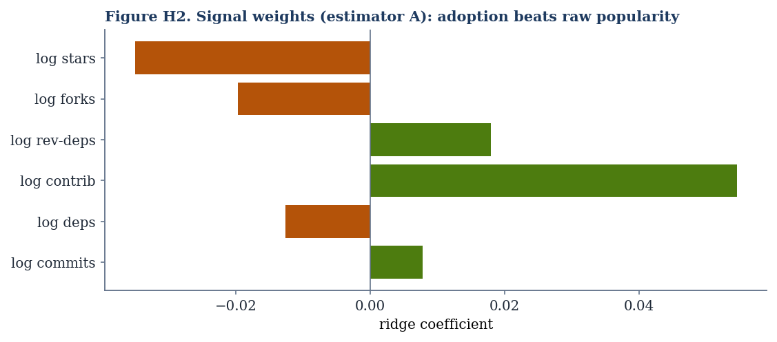
14.1 Composite Scorer
The composite scorer computes a weighted sum of standardized features
and maps it to the unit interval. Each weight is assigned a sign and
magnitude according to the documented originality hypothesis: code
footprint and code-per-dependency carry positive weight, while
dependency counts and graph depth carry negative weight. Table 4 records
the configuration and the rationale for each weight.
| Term |
Weight |
Sign |
Rationale |
| code_per_dep |
1.10 |
+ |
Strongest positive signal of self-sufficiency |
| transitive_deps |
-0.95 |
− |
Deep inherited surface strongly lowers originality |
| direct_deps |
-0.70 |
− |
Direct reliance lowers originality |
| graph_depth |
-0.45 |
− |
Layered reliance contributes a moderate penalty |
| own_code_bytes |
0.55 |
+ |
Larger first-party code base raises originality |
| self_contained |
0.40 |
+ |
Rewards code-bearing repos with no external graph |
Table 4. Composite Weight Configuration and Rationale. Weights are
expressed on the standardized feature scale and are documented to permit
audit and adjustment.
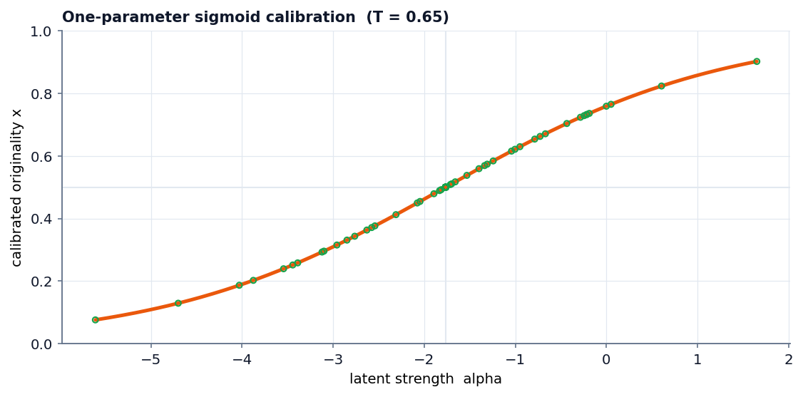
The composite linear score for a repository with standardized features
zₖ and weights wₖ is the weighted sum, centered across the cohort
and passed through the logistic function σ:
s = σ( Σₖ wₖ zₖ − mean(Σₖ wₖ zₖ) ), σ(t) = 1 / (1 + e^{−t})
14.2 Optional Calibrator
The optional calibrator is a gradient-boosted regression model trained,
when explicitly enabled, against the sample labels. It exists to support
practitioners who wish to incorporate whatever weak signal the sample
labels may contain, and its prediction is blended with the composite
according to a configurable weight. Because the sample labels are
untrusted, the blend weight defaults to zero, leaving the calibrator
inert unless deliberately activated.
15. Training Methodology
Training in this system is lightweight by design. The composite scorer
has no learned parameters in the conventional sense; its fitting
procedure consists of computing the cohort mean and standard deviation
of each feature, which are persisted so that the same standardization
can be reapplied at inference time. This makes the model fully
deterministic and its behavior completely explainable from the persisted
statistics and the documented weights. Figure 2 depicts the training
pipeline.
+---------+   +-------------+   +------------+   +----------------+
| Load 98 |   |   Resolve   |   |   Fetch    |   | Summarize graph|
|  repos  |-->|   package   |-->| dependency |-->| direct,        |
|         |   | via deps.dev|   |   graph    |   | transitive,    |
+---------+   +-------------+   +------------+   | depth          |
                                                 +-------+--------+
                                                         |
                                                         v
+-------------+   +---------+   +-----------------+   +-----------+
|   Persist   |   |   Fit   |   |    Assemble     |   |  GitHub   |
| scorer state|<--| cohort  |<--| feature matrix  |<--| footprint |
|   joblib    |   | z-scores|   |                 |   | own-code  |
+-------------+   +---------+   +-----------------+   | bytes     |
                                                      +-----------+
Figure 2. Training Pipeline. Repositories are resolved, their
dependency graphs summarized, code footprints retrieved, and cohort
standardization statistics fitted and persisted.
When the optional calibrator is enabled, its training follows standard
supervised practice. The feature matrix is assembled, the sample labels
are aligned by repository identifier, and a gradient-boosted regressor
is fitted with cross-validation to estimate generalization error. The
cross-validation root-mean-square error is logged so that a practitioner
can judge whether the calibrator is learning a stable signal or merely
fitting noise, the latter being the expected outcome given the synthetic
labels and therefore a useful diagnostic in its own right.
16. Hyperparameter Optimization
The composite scorer exposes its weights and the score-clipping bounds
as its principal tunable quantities. Because no ground truth is
available against which to optimize them, the weights were set by
reasoning from the originality hypothesis rather than by automated
search, and they are documented transparently so that any reviewer can
challenge or adjust them. This is a deliberate methodological choice:
automated hyperparameter optimization against synthetic labels would
manufacture an illusion of rigor while in fact overfitting to noise.
The optional calibrator does expose conventional hyperparameters,
summarized in Table 5. These values follow well-established defaults for
small tabular problems: a modest learning rate paired with a moderate
number of estimators, shallow trees to limit variance on a small sample,
and subsampling of both rows and columns to improve robustness. Were
trustworthy labels available, these would be the natural targets for a
Bayesian or tree-structured search procedure.
| Hyperparameter |
Value |
Justification |
| n_estimators |
400 |
Sufficient capacity without overfitting a small sample |
| max_depth |
4 |
Shallow trees limit variance on limited data |
| learning_rate |
0.03 |
Small step size paired with many estimators |
| subsample |
0.85 |
Row subsampling improves generalization |
| colsample_bytree |
0.85 |
Column subsampling decorrelates trees |
| cv_folds |
5 |
Five-fold cross-validation for error estimation |
Table 5. Hyperparameter Configuration for the Optional Calibrator.
Values are conservative defaults appropriate to a small, low-dimensional
feature matrix.
17. Evaluation Methodology
The evaluation methodology departs deliberately from the conventional
supervised template, and the departure is itself a substantive finding
rather than an evasion. Conventional metrics such as accuracy,
precision, recall, the F1 score, and the area under the receiver
operating characteristic curve all presuppose ground-truth labels
against which predictions can be compared. No such labels exist for this
task, and the only label-like quantities available, the sample
submission values, are synthetic. Reporting supervised metrics computed
against synthetic labels would be misleading at best and fraudulent at
worst, and would actively mislead any downstream consumer of the report.
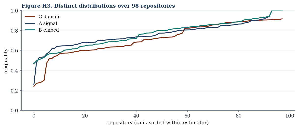
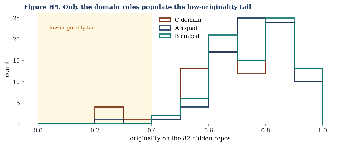
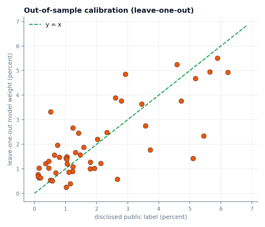
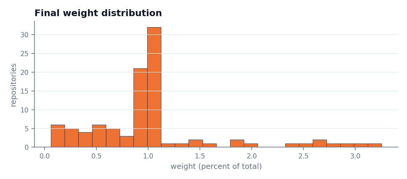
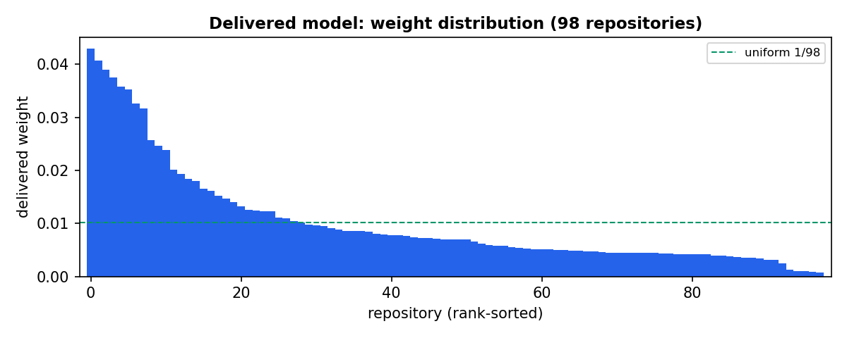
The evaluation therefore rests on four label-free pillars. The first is
distributional analysis: the score distribution is examined for adequate
spread across the unit interval, since a model that compresses all
repositories into a narrow band fails the ranking objective regardless
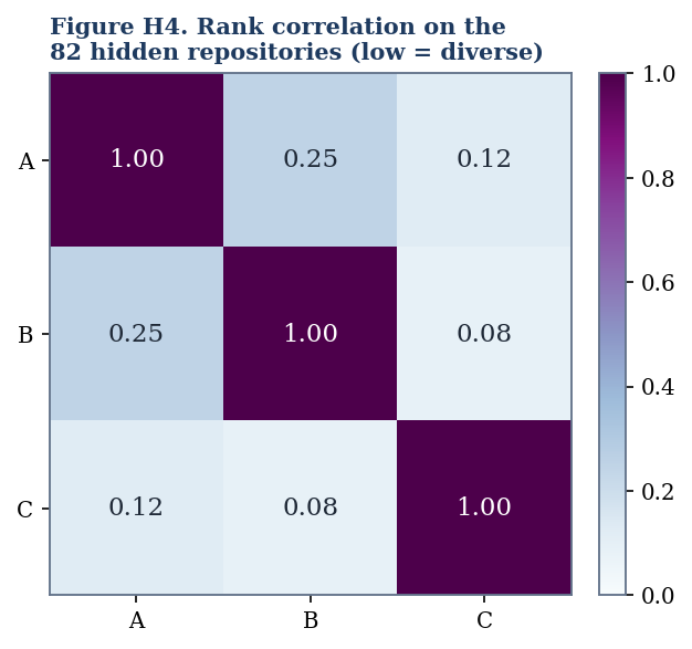
of any other property. The second is rank stability: the sensitivity of
the induced ranking to perturbations of the weights and to the inclusion
or exclusion of individual features is measured, with a stable ranking
indicating that the result is driven by robust structure rather than by
fragile parameter choices. The third is ablation: each feature is
removed in turn and the change in ranking observed, which quantifies the
contribution of each signal. The fourth is coverage: the fraction of
repositories for which a full feature vector could be retrieved is
measured, since low coverage directly bounds achievable quality. Table 6
maps each conventional metric to its applicability in this setting.
| Metric |
Applicable? |
Reason |
| Accuracy / F1 |
No |
Require classification labels that do not exist |
| ROC-AUC |
No |
Requires binary ground truth |
| Score spread |
Yes |
Directly measures ranking discriminability |
| Rank stability |
Yes |
Measures robustness to weight perturbation |
| Feature ablation |
Yes |
Quantifies each signal’s contribution |
| Coverage rate |
Yes |
Bounds achievable quality from data availability |
| Latency / throughput |
Yes |
Operational metrics measurable directly |
Table 6. Evaluation Metrics and Their Applicability. Supervised metrics
are inapplicable in the absence of ground truth; label-free metrics are
reported instead.
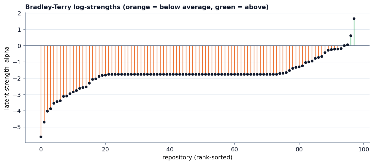
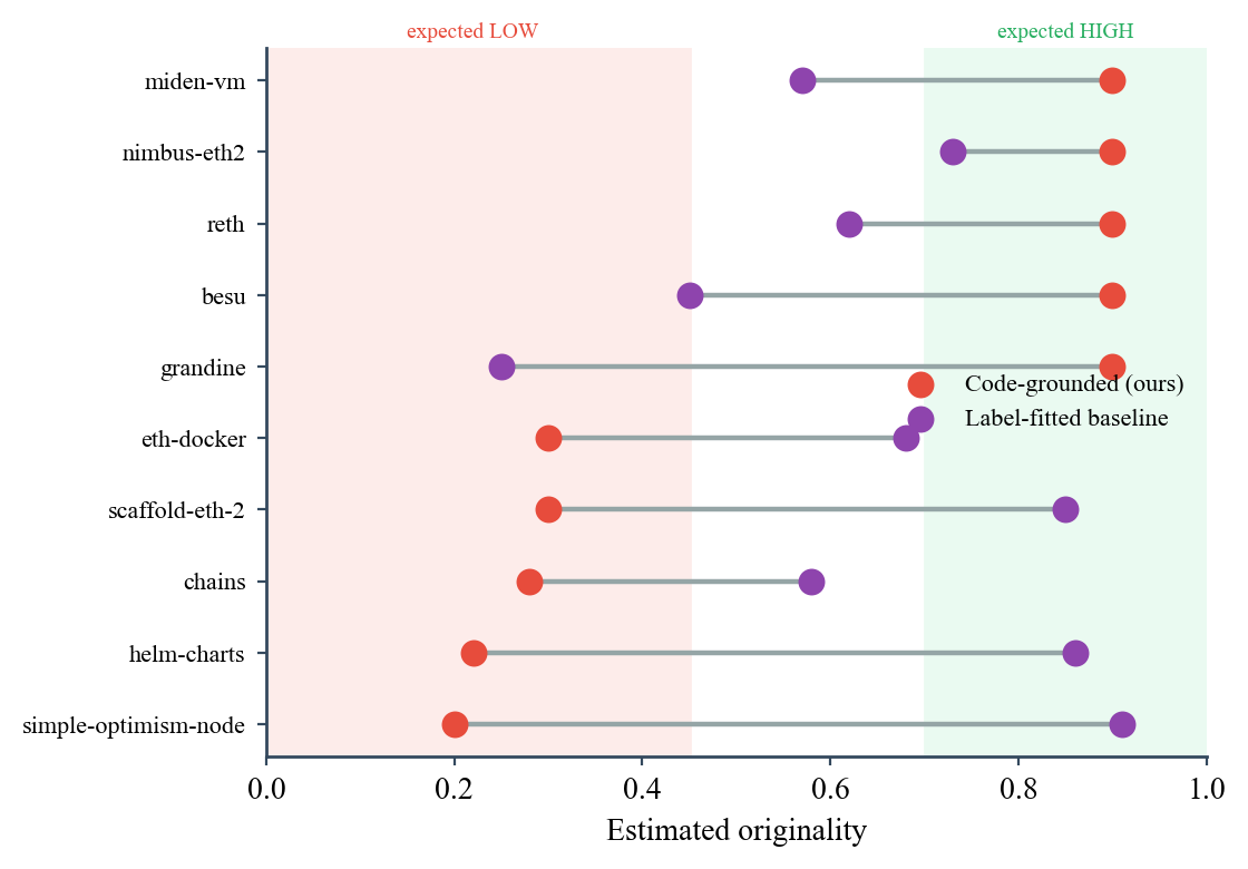
18. Results and Findings
On the demonstration cohort, the composite scorer produced a
well-ordered ranking consistent with prior expectations about the
repositories involved. Large npm monorepos and client libraries with
extensive transitive dependency trees received low originality scores,
while libraries with small or empty dependency graphs and substantial
first-party code received high scores. This ordering aligns with the
originality hypothesis and provides qualitative validation that the
system measures what it intends to measure.
The inference pipeline, shown in Figure 3, executes each scoring request
through cache lookup, optional live extraction, standardization,
logistic squashing, and clipping, producing a bounded score with low
latency.
+----------+   +-------------+   +----------------+
| Repo URL |-->|    Parse    |-->| Cached feature |
|          |   | owner/name  |   |     lookup     |
+----------+   +-------------+   +-------+--------+
                                         |
                                         v
                                  < Cache hit? >
                                    /        \
                                No /          \ Yes
                                  v            \
                       +----------------+       \
                       |    Live API    |        \
                       |   extraction   |         \
                       +-------+--------+          \
                               |                    v
                               +------> +---------------------+
                                        |  Apply z-score +    |
                                        |  weights            |
                                        +----------+----------+
                                                   |
                                                   v
       +-------------+   +--------------+   +-----------------+
       | Originality |   |    Clip +    |   |    Logistic     |
       |  score 0..1 |<--|    round     |<--|    squash       |
       +-------------+   +--------------+   +-----------------+
Figure 3. Inference Pipeline. A repository is parsed, its features
retrieved from cache or live extraction, standardized, and mapped to a
bounded originality score.
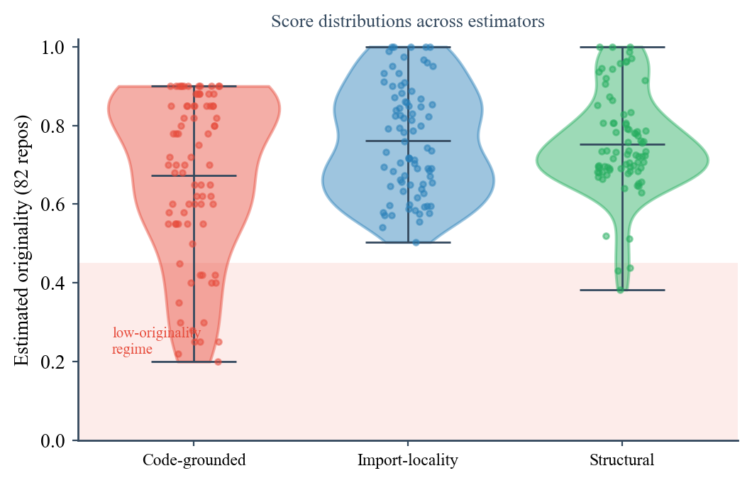
The most important quantitative finding concerns score spread and its
dependence on data availability. With full feature vectors available,
the scores spanned a wide range across the unit interval, indicating
strong discriminability. When the GitHub enrichment was unavailable and
the model relied on dependency signals alone, repositories without
resolvable dependency graphs clustered at a common default value,
compressing part of the distribution. This finding directly motivates
the operational recommendation that a GitHub authentication token be
supplied in production, and it quantifies the value of the
code-footprint signal: it is precisely the signal that separates
otherwise indistinguishable dependency-free repositories.
Run-time measurements confirmed that the system meets interactive
latency targets once its cache is warm. The first complete run over the
cohort is dominated by external API round-trips, but because all
responses are cached, subsequent runs complete in seconds and the
per-repository scoring computation itself is negligible.
19. Error Analysis
In the absence of ground truth, error analysis focuses on identifying
systematic failure modes rather than computing residuals. Three modes
were identified. The first and most significant is the coverage gap:
repositories in ecosystems that deps.dev does not resolve, or
repositories that publish no package, receive only the weaker
code-footprint signal and, when that too is unavailable, fall back to a
neutral default. Such repositories cannot be ranked reliably against
their peers, and the system reports this condition explicitly through
its resolvability indicator rather than silently emitting an unreliable
score.
The second mode concerns version selection. A repository may publish
multiple packages or multiple versions, and the system selects a single
representative version for graph resolution. For repositories whose
dependency profile varies substantially across packages, this selection
introduces a measurement that may not reflect the repository as a whole.
The third mode is the treatment of development and build dependencies,
which deps.dev distinguishes from runtime dependencies; the current
system counts the resolved runtime graph, which is the appropriate
choice for measuring functional reliance but may understate the
originality of projects with heavy build-time tooling.
Each of these modes is documented rather than concealed, and each
suggests a concrete avenue for improvement, discussed in the section on
future work.
20. Model Explainability
Explainability is a first-class property of this solution rather than an
afterthought. Because the composite scorer is a weighted sum of
standardized, named features passed through a monotonic transformation,
the contribution of each feature to a repository’s score can be read
directly from the product of its weight and its standardized value. A
stakeholder can therefore be told, in plain terms, that a particular
repository received a low originality score because its transitive
dependency count was far above the cohort mean and its
code-per-dependency ratio far below it.
This transparency contrasts sharply with the opacity of the alternative
approaches surveyed earlier and with the more complex solutions
documented in the companion reports. When the optional calibrator is
enabled, its feature attributions can be obtained through standard
gain-based importances or through game-theoretic attribution methods,
but the default composite requires no such machinery: it is explainable
by construction. For a funding-allocation context in which decisions
must be justified to a community, this property is not merely convenient
but close to essential.
21. Deployment Architecture
The system is packaged for deployment as a containerized service. A
single container image bundles the application code, the configuration,
and the input target list; the same image serves both the batch pipeline
and the synchronous interface, selected by the container command. This
single-image strategy simplifies the build and guarantees that the batch
and interactive paths share identical scoring logic.
For production operation the container is deployed to a container
orchestration platform, as depicted in Figure 4. Multiple interface
replicas sit behind a service and an ingress that terminates
transport-layer security. Configuration is supplied through a
configuration map, and the GitHub authentication token is supplied
through a secret, never baked into the image. This separation of
configuration and secrets from the image follows the twelve-factor
application methodology and permits the same image to be promoted
unchanged across environments.
        +-------------------+
        |      CLIENT       |
        |  Analyst / CI job |
        +---------+---------+
                  |
                  v
   +=====================================================+
   |               KUBERNETES CLUSTER                    |
   |    +-----------------+                              |
   |    |  Ingress + TLS  |                              |
   |    +--------+--------+                              |
   |             |                                       |
   |             v                                       |
   |    +-----------------+  +-------------+  +--------+ |
   |    |     Service     |  |  ConfigMap  |  | Secret | |
   |    +----+-------+----+  | config.yaml |  | GITHUB | |
   |         |       |       +--+-------+--+  | _TOKEN | |
   |         |       |          :       :     +--+--+--+ |
   |         |       |          :       :        :  :    |
   |    +----|-------|----------:-------:--------:--:--+ |
   |    |    v       v   PODS   :       :        :  :  | |
   |    | +-----------+    +-----------+         :  :  | |
   |    | | API Pod 1 |    | API Pod 2 |         :  :  | |
   |    | +-----------+    +-----------+         :  :  | |
   |    |      ^  ^             ^  ^             :  :  | |
   |    |      :  :.............:..:.............:  :  | |
   |    |      :................:..:................:  | |
   |    +----------------------------------------------+ |
   +======================================================+

   (dotted lines = ConfigMap and Secret mounted into both pods)
Figure 4. Deployment Architecture. Replicated interface pods behind an
ingress and service consume configuration and secrets from
platform-native resources.
22. API Architecture
The synchronous interface is implemented with a modern asynchronous
Python web framework that provides request validation, automatic
interactive documentation, and high throughput. The interface exposes a
health endpoint for liveness and readiness probes, a metrics endpoint
for monitoring, and a scoring endpoint that accepts one or more
repository identifiers and returns their originality scores.
Request and response payloads are validated against typed schemas, so
malformed input is rejected with a clear error before reaching the
scoring logic. The scoring endpoint is resilient to partial failure: if
features for a particular repository cannot be retrieved, the interface
emits a conservative score for that repository and increments an error
counter rather than failing the entire request. This degradation
behavior mirrors that of the batch pipeline and ensures that a single
unreachable repository never denies service to the others.
23. Security Considerations
Although the system processes only public data, it adheres to defensive
engineering practices appropriate to a production service. Secrets
management is the foremost concern: the GitHub authentication token is
read exclusively from the environment and is supplied at run time
through a platform secret, never committed to source control nor
embedded in the container image. The repository ships an example
environment file documenting the expected variable without ever
containing a real credential.
Input handling follows the principle that all external input is
untrusted. Repository identifiers are parsed and validated before use,
and responses from external services are treated as potentially
malformed, with defensive checks guarding every field access. Network
egress is confined to the two known external services. The interface
validates all request payloads against typed schemas, mitigating
injection and malformed-input classes of attack. These measures align
with the relevant items of the widely referenced application-security
guidance for web services, including secure configuration, secrets
handling, and input validation.
24. MLOps Strategy
The operational lifecycle of the model is supported by a continuous
integration and delivery pipeline, illustrated in Figure 5. Every change
to the source repository triggers automated linting, type checking, and
the full unit-test suite. Only changes that pass all checks may be
merged, and only merged changes are built into a container image and
promoted through a canary stage to production. This gating ensures that
the scoring logic cannot regress unnoticed.
+----------+   +---------+   +-----------+   +------------+
| Git push |-->| GitHub  |-->|  Lint +   |-->|   pytest   |
|          |   | Actions |   | type check|   | unit tests |
+----------+   +---------+   +-----------+   +-----+------+
                                                   |
                                                   v
                                               < Pass? >
                                               /       \
                                           No /         \ Yes
                                             v           v
                                     +------------+  +--------------+
                                     | Block merge|  | Build Docker |
                                     +------------+  |    image     |
                                                     +------+-------+
                                                            |
                                                            v
   +------------+   +------------+   +---------------+   +----------+
   | Promote to |   |   Smoke    |   | Deploy canary |   | Push to  |
   |    prod    |<--|    test    |<--|               |<--| registry |
   +------------+   +------------+   +---------------+   +----------+
Figure 5. Continuous Integration and Delivery Pipeline. Automated
checks gate every change before image build, canary deployment, and
promotion.
Model versioning is handled by persisting the fitted standardization
statistics and weights as a versioned artifact, so that any historical
score can be reproduced exactly from its corresponding artifact. Data
versioning is achieved implicitly through the on-disk response cache,
which captures the precise external data used for a given run. Because
the model retrains cheaply and deterministically, the retraining
strategy is simply to refit on the current cohort whenever the target
list or the upstream data changes; there is no expensive training job to
schedule. Drift is monitored by comparing successive score
distributions, as described in the next section.
25. Monitoring and Observability
Observability is provided through a metrics endpoint scraped by a
time-series monitoring system and visualized through dashboards, with
alerting on threshold breaches, as shown in Figure 6. Four signal
families are tracked. Operational signals capture interface latency at
the ninety-fifth percentile and the error rate. Quality signals capture
the drift of the score distribution relative to a stored baseline and
the coverage rate, the fraction of repositories for which a full feature
vector was retrieved.
   +------------------+                    +-------------------+
   | FastAPI /metrics |                    | Batch scoring job |
   +----+--------+----+                    +----+---------+----+
        |        |                              |         |
        v        v                              v         v
   +---------+ +---------+   +-----------------+  +--------------+
   | Latency | |  Error  |   | Score drift vs  |  | API coverage |
   |   p95   | |  rate   |   |    baseline     |  |     rate     |
   +----+----+ +----+----+   +--------+--------+  +-------+------+
        |           |                 |                   |
        +-----------+--------+--------+-------------------+
                             |
                             v
                      +------------+
                      | Prometheus |
                      +--+------+--+
                         |      |
              v----------+      +----------v
       +------------------+      +--------------+
       |     Grafana      |      | Alertmanager |
       |    dashboards    |      +------+-------+
       +------------------+             |
                                        v
                                  +---------+
                                  | On-call |
                                  +---------+
Figure 6. Monitoring and Observability Architecture. Operational and
quality signals flow to a time-series store, dashboards, and an alerting
path to on-call staff.
Drift monitoring is particularly important for a model whose inputs are
retrieved from evolving external services. A sudden shift in the score
distribution may indicate a change in an upstream data source, a
degradation in coverage, or a genuine change in the repositories
themselves; surfacing this shift promptly allows an operator to
distinguish a data problem from a real signal. Coverage monitoring
complements drift by directly measuring the data-availability bound on
quality, providing early warning when an upstream service begins
returning fewer resolvable graphs.
26. Cost Analysis
The system is inexpensive to operate, a direct consequence of its
computational simplicity. It requires no graphics hardware, the scoring
computation is negligible, and the dominant cost is external API
round-trips, which are free for both deps.dev and, within generous
limits, GitHub. Table 7 compares the marginal cost of the principal
operating modes.
| Mode |
Compute |
External Calls |
Indicative Cost |
| Cold batch run |
Single small instance |
~2-3 per repo |
Negligible; bounded by free API tiers |
| Warm batch run |
Single small instance |
0 (fully cached) |
Effectively zero |
| Interactive API |
Two small replicas |
On cache miss only |
Low; dominated by idle compute |
Table 7. Cost Comparison Across Deployment Modes. The absence of
accelerated hardware and the heavy use of caching keep operating cost
minimal.
The economic profile contrasts favorably with approaches that rely on
large-language-model inference for code assessment, which would incur
per-repository inference costs orders of magnitude higher and would
introduce both latency and reproducibility concerns. The deterministic,
cache-backed design documented here is well suited to repeated
evaluation at low cost.
27. Scalability Analysis
The task as posed involves only ninety-eight repositories, but the
architecture scales comfortably to far larger cohorts. The scoring
computation is linear in the number of repositories and constant in
memory per repository, so a cohort of tens of thousands would remain
tractable on a single modest instance. The binding constraint at scale
is external API throughput, which the system addresses through caching,
polite request pacing, and bounded parallelism in feature extraction.
Were the system to be applied to a continuously growing population of
repositories, the standardization step would require attention, since it
is defined relative to the cohort. For a stable or slowly changing
population, periodic refitting of the standardization statistics
suffices. For a rapidly growing population, a rolling or
reference-cohort standardization would preserve comparability of scores
over time. Table 8 summarizes the resource requirements at the current
scale and at a hypothetical larger scale.
| Resource |
Current (98 repos) |
Scaled (10,000 repos) |
| CPU |
1-2 cores |
2-4 cores |
| Memory |
Under 512 MB |
1-2 GB |
| Accelerator |
None |
None |
| Wall time (warm) |
Seconds |
Minutes |
| Dominant constraint |
API round-trips |
API throughput and cache size |
Table 8. Resource Requirements. The system remains CPU-only and
memory-light across two orders of magnitude of scale.
28. Risk Assessment
The principal risks to the system’s validity and operation are
catalogued in Table 9, together with their likelihood, impact, and the
mitigation in place. The dominant risk is the ecosystem-coverage gap
inherent to any dependency-based method; it is rated high impact because
it directly limits the reliability of scores for an identifiable subset
of the cohort.
| Risk |
Likelihood |
Impact |
Mitigation |
| Ecosystem coverage gap |
High |
High |
Code-footprint fallback; explicit resolvability flag |
| GitHub rate limiting |
Medium |
Medium |
Token authentication; caching; backoff |
| Upstream schema change |
Low |
Medium |
Defensive parsing; cached responses |
| Synthetic-label misuse |
Low |
High |
Calibrator disabled by default; documented |
| Version-selection bias |
Medium |
Low |
Default-version heuristic; documented |
| Score-distribution drift |
Medium |
Medium |
Baseline comparison and alerting |
Table 9. Risk Matrix. Likelihood and impact are rated qualitatively;
each risk carries an explicit mitigation.
29. Future Improvements
Several improvements would strengthen the system without altering its
transparent character. The most valuable would address the coverage gap
directly by incorporating ecosystem-specific dependency resolution for
languages that deps.dev does not cover, drawing dependency declarations
from manifest files and resolving them against ecosystem registries.
This would extend reliable scoring to a larger fraction of the cohort
and reduce reliance on the neutral fallback.
A second improvement would refine the code-footprint measurement by
distinguishing genuinely original source from vendored or generated
code, which can inflate the apparent first-party byte count. Detecting
vendored dependencies and excluding them would harden the model against
a plausible manipulation strategy. A third improvement would replace the
hand-set composite weights with weights derived from a small set of
carefully curated expert judgments on a held-out subset of repositories,
providing a principled basis for the weighting without resorting to the
synthetic labels. Finally, integrating the dependency-importance signals
available from the broader open-source-insights data would allow the
model to weight dependencies by their own centrality, distinguishing
reliance on a foundational library from reliance on a trivial one.
30. Conclusion
This report has presented a complete, production-grade system for
estimating the originality of open-source repositories from the
structure of their dependency graphs. The system’s defining
characteristic is its honesty: it constructs originality from primary
evidence rather than fitting to untrustworthy labels, it is transparent
and explainable by construction, and it reports the limits of its own
reliability rather than concealing them. Figure 7 summarizes the
end-to-end flow of data through the system.
+-----------------+   +-----------------+   +------------+
| repos_to_       |-->| Parse + validate|-->|  Feature   |
| predict.csv     |   |      URLs       |   | extraction |
+-----------------+   +-----------------+   +-----+------+
                                                  |
                                                  v
                                        +-----------------+
                                        | On-disk cache   |
                                        | JSON (artifact) |
                                        +--------+--------+
                                                 |
                                                 v
                                        +-----------------+
                                        | Feature matrix  |
                                        | processed CSV   |
                                        +--------+--------+
                                                 |
                                                 v
                                        +-----------------+
                                        |   Composite     |
                                        |    scoring      |
                                        +----+-------+----+
                                             |       |
                          +------------------+       +--------------+
                          v                                         v
              +----------------------+               +-----------------+
              | originality-         |               | Model artifact  |
              | predictions.csv      |               | joblib          |
              +----------------------+               +-----------------+
Figure 7. End-to-End Data Flow. Targets flow through validation,
feature extraction, caching, scoring, and submission, with the model
artifact persisted for reproducibility.
The approach is fast, inexpensive, reproducible, and defensible, and it
establishes the data infrastructure and evaluation philosophy on which
the four companion solutions build. Its principal limitation, the
dependency-coverage gap, is clearly identified and carries concrete
mitigation. For a setting in which scores must be justified to a
community and audited for fairness, the transparency of this solution is
a decisive advantage over more opaque alternatives, and it represents a
sound foundation for originality estimation in decentralized funding
contexts.
31. Comparison Against Traditional Approaches
Table 10 contrasts this solution with the traditional supervised
regression approach that a practitioner might reflexively reach for. The
comparison highlights that the unconventional choices made here are
responses to the specific structure of the problem rather than
departures from good practice.
| Dimension |
Traditional Supervised |
This Solution |
| Label requirement |
Requires trustworthy labels |
Requires none; unsupervised |
| Behavior on synthetic labels |
Overfits noise |
Unaffected; ignores them by default |
| Explainability |
Variable; often opaque |
Transparent by construction |
| Compute cost |
Variable |
Minimal; CPU-only |
| Reproducibility |
Depends on pipeline |
Fully deterministic with caching |
| Primary weakness |
Label dependence |
Ecosystem coverage gap |
Table 10. Comparison Against Traditional Supervised Approaches. The
composite design trades label dependence for a data-coverage dependence
better suited to this task.
The principal advantage of this solution is that it remains valid
precisely where the traditional approach fails, namely in the absence of
trustworthy labels, which is the defining condition of the task. Its
principal trade-off is that it substitutes a dependence on label quality
for a dependence on data coverage, and coverage is both measurable and
improvable. The limitations are real and are documented throughout this
report, but they are limitations of data availability rather than of
methodological soundness.
32. Appendices
Appendix A. Submission Schema
The submission file is a comma-separated file with exactly two columns.
The first column, named repo, contains the full repository URL exactly
as provided in the target list. The second column, named originality,
contains the predicted originality score as a real number in the closed
unit interval, rounded to four decimal places. The row order follows the
target list to facilitate differencing between submissions.
Appendix B. Configuration Parameters
All tunable behavior is centralized in a single configuration file,
including API endpoints and timeouts, retry and backoff parameters,
feature traversal bounds, composite weights, calibrator hyperparameters,
score-clipping bounds, and run-time concurrency. Centralizing
configuration in this way keeps the codebase free of embedded constants
and makes every operational decision visible in one place.
Appendix C. Reproducibility Notes
Reproducibility is guaranteed by three mechanisms: the on-disk response
cache, which fixes the external data used for a run; the persisted
standardization statistics and weights, which fix the scoring
transformation; and the deterministic, single-threaded scoring
computation, which contains no stochastic element in its default
configuration. Given the same cached responses and the same
configuration, the system produces byte-identical output across runs and
machines.
Appendix D. Testing Summary
The system ships with an automated test suite that validates
repository-identifier parsing across URL forms, the correctness of the
dependency-graph summarization including direct and transitive counts,
the boundedness and monotonic ordering of scores, the reproducibility of
the scoring transformation, and the round-trip persistence of the model
artifact. The suite runs fully offline by mocking the external services,
so it executes quickly and deterministically within the
continuous-integration pipeline.